The following script generates and saves the electrostatic potential data.
#######################################################
## Tutorial by: Andrew
## Topic: Electrostatic potential in ase-espresso
##
## dependencies: ase, espresso, pickle
##
## Generates the data files necessary to analyze
## the charge density and electrostatic potential
## in and around a Pt(100) slab
#######################################################

# Import necessary packages
from ase import Atoms
from ase.io import write
from ase.lattice.surface import fcc100
from espresso import espresso
import pickle

# Generate the representation of the atoms in ASE
slab = fcc100('Pt', size=(2,2,3), vacuum=10.0)

# Create an espresso calculator object
# (Tailor for desired settings and accuracy)
calc = espresso(pw=400 , # Plane wave cutoff
                dw=4000, # Density wave cutoff
                kpts=(3,3,1), # (rather sparse) k-point (Brillouin) sampling
                xc='RPBE', #Exchange-correlation functional
                dipole={'status':True}, # Includes dipole correction (necessary for asymmetric slabs)
                outdir='pt100_analysis') # Espresso-generated files will be put here

# Attach the calculator object to the atoms
slab.set_calculator(calc)

# Perform a static calculation to generate wavefunctions
slab.get_potential_energy()

# Create an image of the atoms
write('slab.png',slab)

# Get the electrostatic potential
potential = calc.extract_total_potential()

# Create and populate output file for electrostatic potential

potential_file=open('potential.pickle','w')
pickle.dump(potential,potential_file)
potential_file.close()
Now we are done with the intensive calculations. The following scripts will interpret the results and can be run easily on any computer in a matter of seconds.
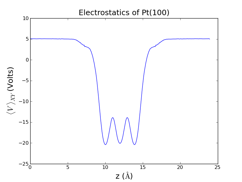
#######################################################
## Tutorial by: Andrew
## Topic: Plotting electrostatic potential data from
##        ase-espresso
##
## dependencies: pickle, pylab, numpy
##
## Plots an XY-averaged electrostatic potential as
## a function of Z position through and outside
## a Pt(100) slab.
#######################################################

# Import necessary packages
import pickle
import pylab as plt
import numpy as np

# Retrieves the data generated in the previous script
potential_file = open('potential.pickle')
potential = pickle.load(potential_file)

origin=potential[0] # [X0,Y0,Z0] - The positions of the origin of the cell.  Here they are [0,0,0]

cell = potential[1] # [3x3 Matrix] Contains the [x,y,z] components of the 3 cell vectors
cell_x = cell[0][0] # The x component of the first cell vector (Remember: This cell is rectangular)
cell_y = cell[1][1] # The y component of the second cell vector (Remember: This cell is rectangular)
cell_z = cell[2][2] # The z component of the third cell vector (Remember: This cell is rectangular)

v = potential[2] # Contains all real-space potential field points.

#######################################################
## Understanding the architecture of the rest of the
## data can be tricky.  Using the variables presented
## here, V(x,y,z)=v[x][y][z].
##
## First we aim to extract all the information
## available to us, based on numpy's architecture.
#######################################################

n_x = len(v) # Returns the number of entries in the first subset (number of X entries)
n_y = len(v[0]) # Returns the number of entries in the second subset (number of Y entries - choice of '0' was arbitrary)
n_z = len(v[0][0]) # Returns the number of entries in the third subset (number of Z entries - choice of '0' was arbitrary)

potential = [] # Initializes a list for average potentials

# Iterate over all space to average and process potential information
for z in range(n_z):
        temp = 0 # Will serve as a partial sum for averaging purposes
        for x in range(n_x):
                for y in range(n_y):
                        temp+=v[x][y][z] # Sums the potential at all points in an X-Y plane
        temp = temp / (n_x*n_y) # Divides by the total number of points
        potential.append( temp ) # Stores the value for average potential at this Z position

# Translates the indices of points along the Z axis into real-space positions
z_coordinate = np.linspace( 0 , cell_z , n_z )

# Plots the data, formats plot
plt.plot(z_coordinate, potential)
plt.xlabel(r'z ($\AA$)',size=18)
plt.ylabel(r'$\langle V \ \rangle_{XY}$ (Volts)',size=18)
plt.title('Electrostatics of Pt(100)',size=18)

# Display plot
plt.show()
# If you'd prefer to save the plot, highlight the line above and uncomment the line below
#plt.savefig('potential_analysis.png')
The end result should look something like this: